Introduction to chaos
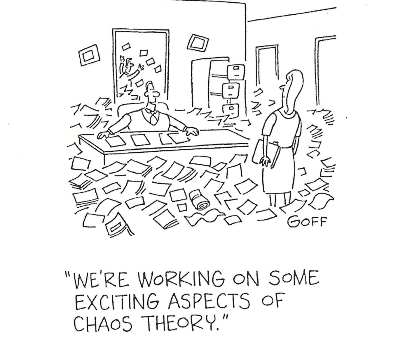
During the eighties, I really got obsessed by a new subject in mathematics, biology, and in physics as well: Chaos Theory. It's about predicting results in chaotic systems, - like the wheather. It turned out that it is practically impossible and that really many things are chaotic, even though we did not realise it in the first place. Just to mention a few:
- Weather
- Stock markets
- Contagious disease
- Earthquake
- Animal population growth
We are used to equations that are Deterministic, - i.e. the result is always the same every time we calculate. It seems obvious. It was actually the invention of the computer that started it all. One of the key issues in the chaos theory is feed back which means that you calculate a result from a deterministic equation and feed that result back into the equation and calculate it one more time and so on many times, i.e. a computer loop. The end result can be quite startling and not what you would expect. The result will change after each calculation but will often come back to the original value and then do the calculation all over again, - it is said to oscillate between results.
If you just want to play around with the bifucation program at the end of this article, click here: Bifucation Program".
In 1961, Lorenz was running a numerical computer model to redo a weather prediction from the middle of the previous run as a shortcut. He entered the initial condition 0.506 from the printout instead of entering the full precision 0.506127 value. The result was a completely different weather scenario.
This is the origin of the phrase The Butterfly Effect. It is important to understand that the "butterfly effect" will only have any effect, if the system is in disequilibrium and can tip to either side. Like if you try to put a pencil on its top. It will eventual fall but you can not predict where.
Bifucation
An australian biologist and mathematician, Robert May, had a hunch that something strange was going on in populations of animals. The populations changed over time. Some years they increased and some years they desceased for no obvious reason. He developed a very simple equation, that was supposed to mimic the fish population in a pond with no interference from outside.
The fish population increased with a certain rate, - let's say by two each year. After a couple of years the population settled on a value that was constant each year. If the fishes were able to increase the population, the population settled on a little higher population.
When he increased the rate to 3 he suddenly saw that the population change each year. Up and down between two values. At 3.5 the periode became 4, at 3.55 the peode was 8. The periode doubled, - a bifufation. After 3.55 the population became chaotic.
Suddenly, at rate 3.829, the population settled on a periode of 3 which then doubled to 6 and further on to 12 and the again chaotic. At a rate of 4 the population of fish became extinct.
Deterministic
This is the essential equation. It is deterministic and liniar but becomes unliniar when it is repeated over time.
r{0 .. 4}
p{0..1}
- First things first: Left side of the equals sign. The equation calculates the next years or seasons population (pn+1) given how many offsprings this population (pn) will produce. "n+1" is the next periode or generation.
-
Right side of the equals sign. Three values are multiplied to give the next population:
"r" is the rate by which the population will increase (or decrease). The interval of the rate is from zero to four. - "p" is the current population. The interval goes from zero to one, - where zero is extinction and one is total over crowded. You can multiply "p" with the maximal population in your population "pond" in order to get the actual population.
- "1 - pn" is included to moderate the growth of the population. If the population approaches 1, - this value will set the result "pn+1" to a very low value. You can say that a big population will eat up all food and be unable to reproduce itself.
Bifucation Diagram
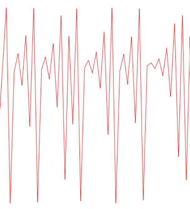
It is very difficult to get an overview of these oscillations,
- especialy when they turn from orderly oscillations to chaotic oscillations.
Robert May came up with another way to show it in a diagram.
He called it a
bifucation diagram.
We know the number of oscillations and the values they fluctuate between. An example could be
a rate at 3.1 and a starting population of 0.5. The population will fluctuate between 0.558 and 0.765.
The only information we need on the diagram is which rate and the population(s). Let us set the rate on the
x-axis and the population(s) on the y-axis. That will be two dots. Then we increase the rate with 0.001 and run the
simulation one more time, draw the dots and so on until the population get extinct, - at a rate of 4.
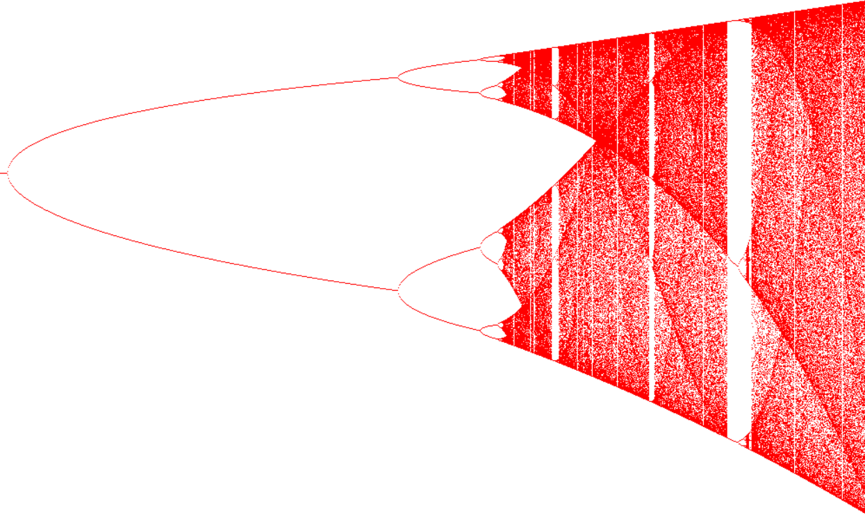
Fractal and recursive
We get the Bifucation Diagram where lines at some rates seem to split into two lines. Further on to the right the same split repeate itself until there are total chaos of dots. These increasingly smaller bifucations are replicas of the bigger ones to the left. They are called fractals and are recursive.
For reasons that I can not explain, there a empty areas in the chaos and they contain new bifucation but now starting at three and then doubled. However, the interval between bifucations are getting incresingly smaller as shown in the table to the right.
Rates and Bifucations
| Rate | Bifucations | Interval |
|---|---|---|
| 2 | 0 | |
| 3 | 2 | |
| 3.45 | 4 | 0.45 |
| 3.545 | 8 | 0.095 |
| 3.5645 | 16 | 0.0195 |
| 3.829 | 3 | |
| 3.841 | 6 | 0.012 |
| 3.8469 | 12 | 0.0059 |
| 3.86 | Chaotic | |
| 4 | Extinction |
Simulation program
You will find a program below that will simulate both the periodes at different rates and make bifucation diagrams.
Diagrams
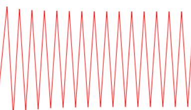
Periode Diagram
The periode can be made several times with different rates and populations. The curves change color in order for you to see the difference between them.
Bifucation Diagram
You can change default rate and population in the input fields as you wish, but start to use the default values, - because they will make the most beautiful bifucation diagram. You can change the default population value of 0.5 but the further it moves away from 0.5 some noise will appear on the graphics due to rounding errors. So just keep it on 0.5.
Press the "Clean" button in order to wipe the board clean.
Warning: It takes some time and CPU-process to create a full bifucation diagram. Up to 40 seconds, depending on the power of your computer. Your browser may warn you that this page slows it down. Just ignore it.
The exact elapsed time will apear below
You must keep the rate between 0 and 5 (values above 4 is extiction) and the population between 0 and 1.
Sources and references